Important Files/Folders that I don't remember the date
The important files/folders inside MG are:
- Background:
- all the withelecmuon* (25000 events);
- Signal:
- truth_studies-master;
- mass_dark_Higgs:
- run_01-03 - Default CMS card (10000 events);
- run_04-06 - CMS card filtered (10000 events);
- run_07-09 - CMS card filtered with btagging change (10000 events);
- signal_mass_dark_Higgs_more_events - CMS card filtered with btagging change (25000 events);
- DM_signal_withelecmuon - CMS card filtered with btagging change (25000 events);
- DM_signal_withelecmuon_change_recojet - CMS card filtered with btagging and jet reco object change (25000 events);
- Files:
- steering.dat;
- run_card.dat;
- param_card.dat;
- ~/Downloads/MG5_aMC_v2_6_4/mass_dark_Higgs/Cards/delphes_card.dat;
The important files inside Delphes are:
- .pdf:
- Background:
- all the withelecmuon* (25000 events);
- Signal:
- all the mass* (10000 events);
- all the filtered_mass* (10000 events);
- all the btag_change_filtered_mass* (10000 events);
- all the more_events_mass* (25000 events);
- all the nojet_mass* (25000 events with the normlepeff* card);
- Macros:
- plot_varios_fjetmass.C;
- maisum_dark_Higgs.C;
- sanity_macro.C;
Important Info
Luminosity for 25000 events (in fb^-1):
- Backgrounds:
- Z: 1454,44;
- W: 439,71;
- Diboson: 489,06;
- top: 476,95;
- Signal:
- m_{hs} = 50 geV - 34,36;
- m_{hs} = 70 geV - 42,20;
- m_{hs} = 90 geV - 51,21;
26/02/2019
Simulated the signal using the CMS card filtered, with the b-tagging eff changed, and with the object to reconstruct the jets also changed. The name of the folder inside the MG folder is
DM_signal_withelecmuon_change_recojet. The ROOT files inside the Delphes folder are named
DM_signal_withelecmuon_change_recojet50.root,
DM_signal_withelecmuon_change_recojet70.root,
DM_signal_withelecmuon_change_recojet90.root. The macros
plot_varios_fjetmass.C and
maisum_dark_Higgs.C were used in those files. The pdf file
fatjet_mass_CMSrecojet.pdf was created.
- The signal was simulated using 25000 events for each mass of the dark Higgs, with the following luminosities (fb^-1):
- m_{hs} = 50 geV - 34,36;
- m_{hs} = 70 geV - 42,20;
- m_{hs} = 90 geV - 51,21.
Changed the
delphes_card.dat to produce the gen fat jets. Started simulating the signal with it to see what happens with the b-tagging. The name of the folder inside the MG folder is
DM_signal_withelecmuon_genfatjet. The ROOT files inside the Delphes folder are named
DM_signal_withelecmuon_genfatjet50,
DM_signal_withelecmuon_genfatjet70,
DM_signal_withelecmuon_genfatjet90. The macros
plot_varios_fjetmass.C and
maisum_dark_Higgs.C were used in those files. The pdf file
fatjet_mass_CMSgenfatjet.pdf was created.
I'll create another macro to analyze the generated fat jets, just like the reconstructed ones to see the differences.
- The signal was simulated using 25000 events for each mass of the dark Higgs, with the following luminosities (fb^-1):
- m_{hs} = 50 geV - 34,36;
- m_{hs} = 70 geV - 42,20;
- m_{hs} = 90 geV - 51,21.
The next step will be to make the b-tagging by hand, that is, try to match the generated b quarks to the jets (gen and reco), and apply the paper eff to it. Also, the test about the random number could be done with one of the masses to check its role in the fat jet invariant mass histograms.
The slides from 25/02/2019 that I showed to Thiago must be changed to be well understood.
08/04/2019
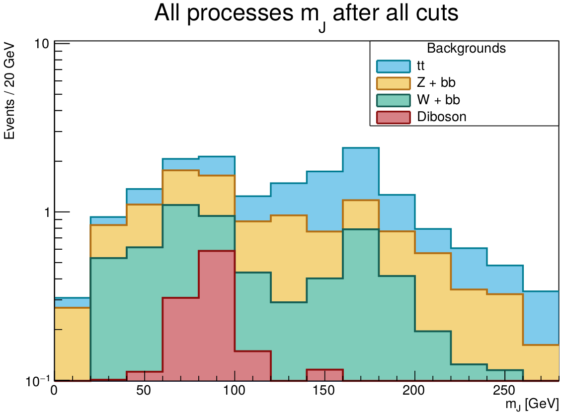
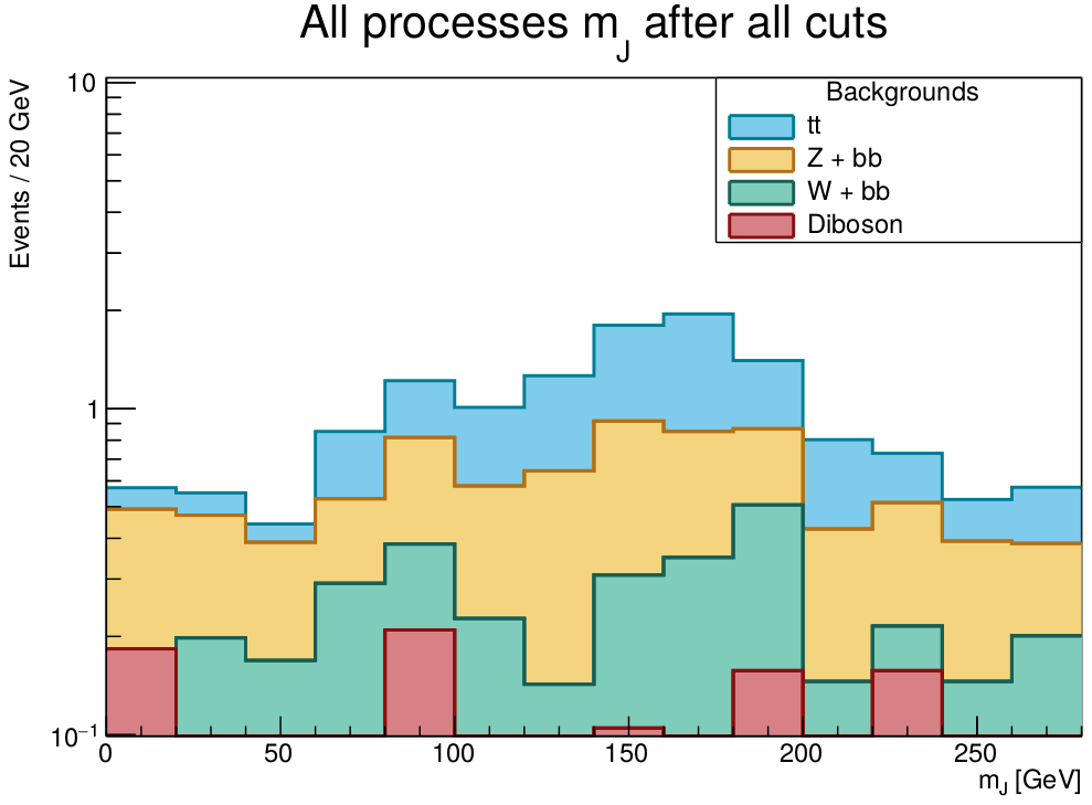
Got a graph exactly like the one in "Hunting the dark Higgs" paper. The name of the file is
ALL_backgrounds_mJ.pdf. Also, the macro used to do it is
ALL_backgrounds_combined_rightratio.C with the files
withelecmuon_ for the backgrounds. I've rescaled the luminosities to 3.2 fb^{-1}, and used a primitive k-factor to do it (choosed 4 because it's the proportion to the ATLAS results). There are some discrepancies between my graph and the paper one that I must talk to Thiago. But it's something.
* bg.png:
 The figure on the left side is from arXiv:1701.08780 [hep-ph].
I've got the right lepton veto using the reconstructed leptons instead of the generated leptons (I guess I was getting ALL of the generated leptons, instead of only the isolated ones). Less then 1% of the signal events were cut using this veto. My problem is still in the b-tagging and the MET cut. The number of events reduced by the MET cut is expected since I'm getting only the end of the tail events (I'll understand this sentence every time). The b-tagging is excluding almost 100% of the signal events, and that is disturbing.
To solve it, I've generated some new signal events TREES from Delphes for the 3 dark Higgs masses (10000 events each), which contain the gen particle, the MET, the jet, gen jet, fat jet, gen fat jet, reco electrons and muons branches to do the b-tagging by hand and check what is happening. The folder is named
DM_signal_withelecmuon_btagging_test, and the files are
DM_signal_withelecmuon_btagging_test50,
DM_signal_withelecmuon_btagging_test70,
DM_signal_withelecmuon_btagging_test90. The macro
genfatjet_macro.C was used in those files.
Also, I've build a macro (
btagging_namao.C) to check Delphes b-tagging and it's WRONG! In the
.root files, there is no b-tagging in the jets, but when I do it by hand, I find a lot (more than zero in this case) of b-tagged jets. I'm testing the jet->Flavor object also, and it seems to be working fine. Don't know what is the problem with Delphes.
The next step is to implement my b-tagging in the real files and get the number of events that pass all of the requirements.
There is another new folder, the
more_events_DM_signal_withelecmuon_btagging_test since 10000 events aren't enough for what I need. Then I'll test the b-tagging again with the gen particles and the jet->Flavor option. The files inside the folder (and in the Delphes folder) are
more_events_DM_signal_withelecmuon_btagging_test50,
more_events_DM_signal_withelecmuon_btagging_test70,
more_events_DM_signal_withelecmuon_btagging_test90 and I've used the macro
btagging_namao.C to check the b-tagging.
These files will be used for the signal number of events prediction.
- The signal was simulated using 30000 events for each mass of the dark Higgs, with the following luminosities (fb^-1):
- m_{hs} = 50 geV - 41,24;
- m_{hs} = 70 geV - 50,64;
- m_{hs} = 90 geV - 61,71.
Tried to solve the NLO problem on
MadGraph, but my knowledge doesn't allow me to do it. Must also talk to Thiago about it. I've even tried to use what CLASHEP taught me, but it didn't worked because there is something else missing.
06/06/2019
I've had some problems generating processes at NLO or using access2, but everything seems to be solved. Apparently the macro for analyzing the events is finished (I HOPE SO), and the results i've already got concerning the dark Higgs events are different from the paper results. I need to show everyone this results at the weekly meeting. 300k events of dark Higgs for each of the masses 50
GeV, 70
GeV and 90
GeV were generated using access2, and the ROOT files are there, and also at my folder /Delphes-3.1.4 and are called
300k_*gev.root.
The NLO processes are difficult to generate, and I'm trying to not follow the paper on this, but it seems very hard. The processes at NLO are
p p > b b~ vl vl~ [QCD] and
p p > b b~ vl l [QCD]. I think that the processes
p p > z z [QCD] and
p p > z w [QCD] with their decays specified in the madspin card, need to be added by hand, since madgraph at NLO is not giving them in the feynman diagrams. The process
p p > b b~ vl vl~ QED<=4 [QCD] gave
ALL the Feynman diagrams, but the software couldn't run (apparently there was some problem in the param_card.dat).
At the meeting (06/06/2019)
I've generated the processes
p p > b b~ vl vl~ and
p p > b b~ vl vl~ QED<=4 at LO, and the diagrams were the same as in the NLO ("the same" reads as their compatible orders). I really need the
QED<=4 part of the syntax, otherwise, diagrams with photons/Higgs will not be accounted for.
I must talk to Thiago about all the problems with the BG at NLO and the signal.
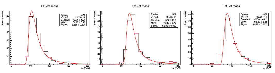
I'm also checking the macro, and there must be a double counting in the b-tagging part. No idea how to solve it. The efficiency of the b-tagging must be inserted in the code, but Thiago will answer this. The graphs for the dark Higgs masses of 50, 70 and 90
GeV are (with a landau fit to get the most probable value of the invariant mass of the fat jets, since it worked better than the other ones (I forgot to put the dark Higgs masses in each of them))
- dh_results.png:
The problem at NLO was solved using the newest version of
MadGraph (2.6.5), with some changes in the files
CT_interface.f. When an process is generated, at the output folder there is the following path
/MG5_aMC_v2_6_5/output_folder/SubProcesses/P0_something_something/V0_something_something/CT_interface.f. Inside those files, approximately at the line 650 (can be higher or lower), two quantities that must be changed are (it's just an extra zero that must be erased)
ABSP_TMP(I)=0.E0+0_16 and
P_TMP(I,J)=0.E0+0_16. The zero after the letter
E must be erased!! Otherwise, the check_poles test will fail.
19/06/2019
I've been talking to Thiago to rewrite the macro, and apparently it's good now, but I'm having problems when applying it to the signal (lots of fat jets have only one jet inside it). The problem seems to be that I forgot to change the
ParameterR variable inside the Delphes card when generating the 300000 events for each mass of the dark Higgs. I've simulated 30000 events of the dark Higgs signal processes for m_{d_{H}} = 50
GeV to check it.
EVERY IMAGE ABOUT THE DARK HIGGS IN THIS TWIKI IS WRONG!!!
The name of the folder is
dh_50gev_30000_paperjetreco, and I'm using the macro (inside Delphes folder)
V3_terceiromais_dark_Higgs.C. I'll also change the way the jets are generated: for now, the jets are reconstructed only using the charged particles (tracks); I'll use the particle flow that includes everything (in Delphes it's the EFlow array).
In the mean time, Thiago taught me how to write a
.root file that contains all the canvases I need, instead of running the macro over and over again (extremely helpful). I also learned how to properly handle data structures in C++, and that save so much time and effort. It makes everything more clear.
Apparently the change in
ParameterR solved the problem. I'll generate 300k events for the 50
GeV dh to check it again. The files will be named
certo_300k_50gev.root and
results_certo_300k_50gev_prunedmass.root (I'll also use the trimmed and the "normal" fat jet masses).
If this work, the masses of 70 GeV and 90 GeV will be tested!
01/07/2019
It seems that everything is working out. My b-tagging is almost exactly like Delphes' one (I only need to include the counting of light quarks, gluons and c jets). I'm getting pretty awesome results that match the paper. Every macro that has the name
V.C* was used to build and test the b-tagging.
V1* and
V2* failed in every aspect.
V3* started to work, but it was a very crude b-tagging, counting some events (read fat jets) that didn't needed to be there.
V4* removed those events, but it was still very crude.
V5* was used to test the cut in
DeltaR (b,j) and worked perfectly.
V6* was already comparing my b-tagging with (spoiler alert!) Delphes B-Tag variable that is working.
V7* is applying the right b-tag efficiency, using a random number to set it (just like the delphes does).
V8* is doing the b-tagging for every jet in the events (light quark and c) with a misidentification efficiency, but it isn't working properly, since the results are very different than those with Delphes b-tag variable.
The signal events are the files with
certo_* .root that were generated following these parameters:
- All of them had m_{\chi} = 100 GeV;
- 300000 events on madgraph run for each;
- All of them were rescaled to L_{r} = 40 fb^-1;
| Mass of the particles |
Luminosity |
Scale factor |
| m_{d_{H}} = 50 GeV, m_{Z'} = 1100 GeV |
L = 411,6244 fb^-1 |
0.0972 |
| m_{d_{H}} = 70 GeV, m_{Z'} = 1100 GeV |
L = 506,0932 fb^-1 |
0.079 |
| m_{d_{H}} = 90 GeV, m_{Z'} = 1100 GeV |
L = 616,9749 fb^-1 |
0.0648 |
| m_{d_{H}} = 70 GeV, m_{Z'} = 625 GeV |
L = 115,4434 fb^-1 |
0.3465 |
| m_{d_{H}} = 70 GeV, m_{Z'} = 1700 GeV |
L = 2633,9161 fb^-1 |
0.0152 |
Besides that, I've figured out why Delphes b-tagging wasn't working, and that is because I don't pay atention to anything. I was overwriting the Reco Jet information with the Gen Jet information, and the Reco Jet weren't being b-tagged, only the Gen Jets. Now I'm generating again the files
mais_certo_* .root with the same prescription as before, and for the m_{d_{H}} = 50
GeV I've already got very nice results. I've also compared my b-tagging with these results, and they are very similar (as they should!).
Don't forget some nice pictures! The next step is to talk to Thiago and check what I'm going to vary to get some efficiencies. Also, I must generate again some backgrounds in NLO to compare with the paper.
Now that all my courses are finished (I hope so) I'll have more time to study C++, python, QFT and HEP.
Below are the images comparing my signal (left images) with the paper signals (right images took from
arXiv:1701.08780 [hep-ph]):
- comp_dh.png:
- comp_Z.png:
02/07/2019
I'm doing all the backgrounds again, and setting up a macro to analyze them, and a signal file just for fun. Apparentely, my old BG results were wrong, since some cuts were missing (lepton isolation variable) or were wrong (I was not getting the fatjet pt or eta after trimming), and I was using the wrong fatjet mass (Delphes default mass before trimming or pruning). The updated/corrected macro for the backgrounds is
mais_certo_ALL_backgrounds_combined_rightratio.C, and a test file was already generated with the name
bgchange_mais_certo_ALL_bg_sig_90gev_withiso.root where I tested the signal with m_{d_{H}} = 90
GeV and some old background process done at LO with the names
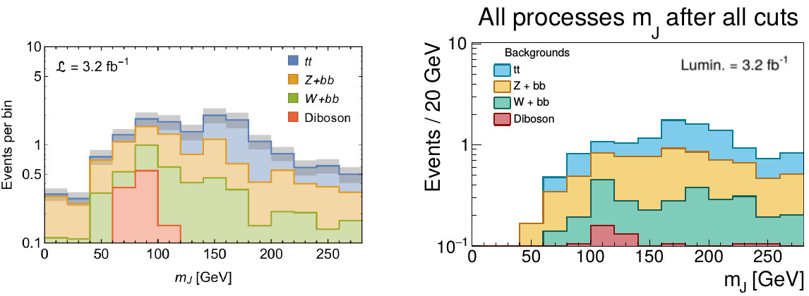
withelecmuon_*. The new result is in the image below (they have the same luminosity, and the figure on the right have a k-factor of 4):
- bg_certo_comp.png:
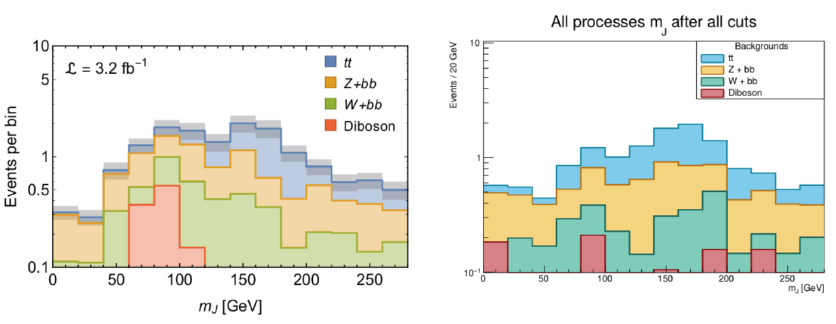
The image on the left was took from arXiv:1701.08780 [hep-ph].
The new BG files will be named
pp2tt_50000_1x.root,
pp2wbb_w2lv_50000_1x.root,
pp2wwbb_50000_1x.root,
NLO_pp2zbb_z2vv_50000_1x.root,
NLO_pp2zz_50000_1x.root and
NLO_pp2wz_50000_1x.root.
I've to remember that there are copies of these files in access 2, including the signal ones that I've talked about on 01/07/2019.
04/07/2019
I've writen a macro to analyze all the 6
.root files for the BG. It's named
NLO_mais_certo_ALL_backgrounds_combined_rightratio.C. I still need to corretly get only the prompt electrons/muons for the lepton veto, but I need to talk to Thiago about this first, since I don't wnat to use the
GenParticle branch of the Delphes tree (It's EXTREMELY slow!!!). The files
ATLAS_kfactors_NLO_bgchange_mais_certo_ALL_bg_sig_90gev_withiso.root and
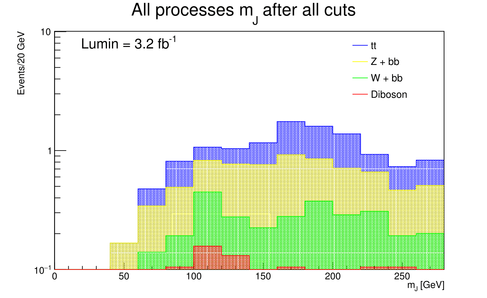
ATLAS_kfactors_NLO_changed_mais_certo_ALL_backgrounds_mJ.pdf have been created using all the right BG, and different k-factors for each background. The results for the number of events of each BG and the ATLAS correspondent comprising the fat jet mass range of 80
GeV to 280
GeV are on the table below:
The comparison of my BG with the paper is in the image below:
- comp_bg_NLO.png:
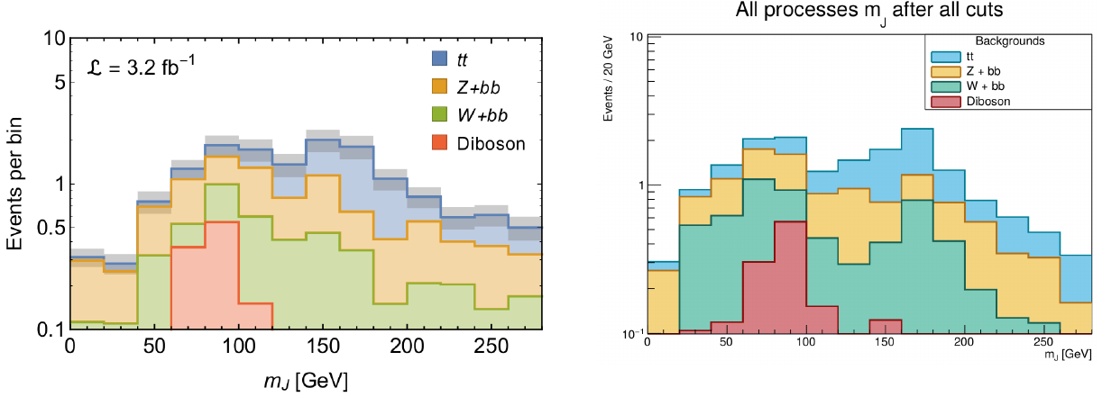
The image on the left was took from arXiv:1701.08780 [hep-ph].
An important factor comes from the madgraph simulation at LO, that accounts for some phenomena that I don't know which it is. Apparentely, if one tries to find the luminosity from the number of generated events and the process cross section, it's 1.2 times smaller than the result of
MadGraph. Unfortunately, at NLO,
MadGraph don't give any luminosity, and it must be calculated usgin this procedure. Using that factor of 1.2 only in the NLO generated BG processes, the new k-factors are:
And the new plot is:
- xsec_factor_bg.png:
09/07/2019
To calculate the efficiencies, I still don't know exactly what to do. I'll perform some tests and talk to Thiago later this week.
To calculate the efficiencies I'll need all processes cross sections, that will be on the table below:
| Process |
x-sec [pb] |
| Dizz |
0.002563 |
| Diwz |
0.001477 |
| Diww |
0.060691 |
| Top |
0.062992 |
| W |
0.221830 |
| Z |
0.137934 |
| 50 |
0.874707 |
| 70 |
0.711139 |
| 90 |
0.583691 |
The macro
punzi_eff_bg_separated.C was created for that, and I'm calculating 2 types of efficiencies: in one of them, I'm summing (BGeff*BGxsec) and then multiplying it by 40000 (that is the luminosity required); in the other one, I'm summing (nBGfin/nBGini), than multiplying by the sum of (BGxsec) and than multiplying by 40000. The punzi eff is being calculated as sigeff/sqrt(1+BG), where BG is (nBGfin/nBGini)*BGxsec*lumin. I'm having some numerical problems since C++ doesn't want to show me the values of the calculations because nfin/nini << 1. I'll try some procedures to make it work.
12/07/2019
In the last days I've been calculating the efficiencies of some cuts in the events. The files are named as
punzieff_something, and the results are pretty impressive. I still need (in some of the graphs of eff_BG x eff_sig) to find the right values of the cuts for each dot.
Besides that, I've talked to Thiago, and we decided to simulate more processes for the dark Higgs signal with different m_{d{H}} and m_{Z'}. The tables below comprise the values of the cross sections for those processes (300k events were simulated for each pair of masses, using access2 from gridunesp):
*m_{Z'} = 1100
GeV, m_{\chi} = 100
GeV:
| m_{d_{H}} [GeV] |
approx x-sec [pb] |
| 50 |
0.874 |
| 60 |
0.788 |
| 70 |
0.711 |
| 80 |
0.643 |
| 90 |
0.583 |
| 100 |
0.530 |
| 110 |
0.477 |
| 120 |
0.410 |
| 130 |
0.325 |
| 140 |
0.222 |
| 150 |
0.118 |
| 160 |
0.0313 |
| 170 |
0.0059 |
| 180 |
0.0037 |
*m_{d_{H}} = 70
GeV, m_{\chi} = 100
GeV:
20/07/2019
First of all, Thiago said about writing a paper!!! I've already checked the works that cited the "Hunting the dark Higgs" (arXiv:1701.08780) paper, and must talk to Thiago about it.
The macro
punzi_eff_bg_separated.C is being used to analyze cuts in the fat jet mass for the m_{d_{H}} = 70
GeV process. I'll do that for the other masses as well. New macros that are called
punzi_eff_metcut.C,
punzi_eff_etacut.C,
punzi_eff_ptcut.C, and
punzi_eff_lepcut.C were created to analyze every other cut. New cuts can be thought of at any time!!!
The macro
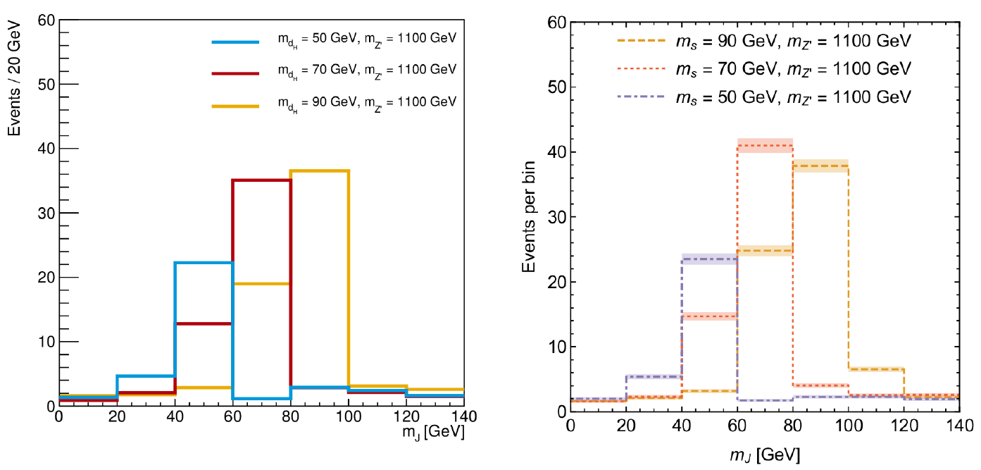
V9_terceiromais_dark_Higgs.C was used at the processes with different m_{d_{H}}. An interesting thing happened at the fat jet ivariant mass from those processes: it had its peak displaced by about 10% for each mass (by comparing the m_{d_{H}} set mass with the m_{J} fitted mass). The graph from the comparison of those masses is in the image below:
- mass_comp_ALL.png:
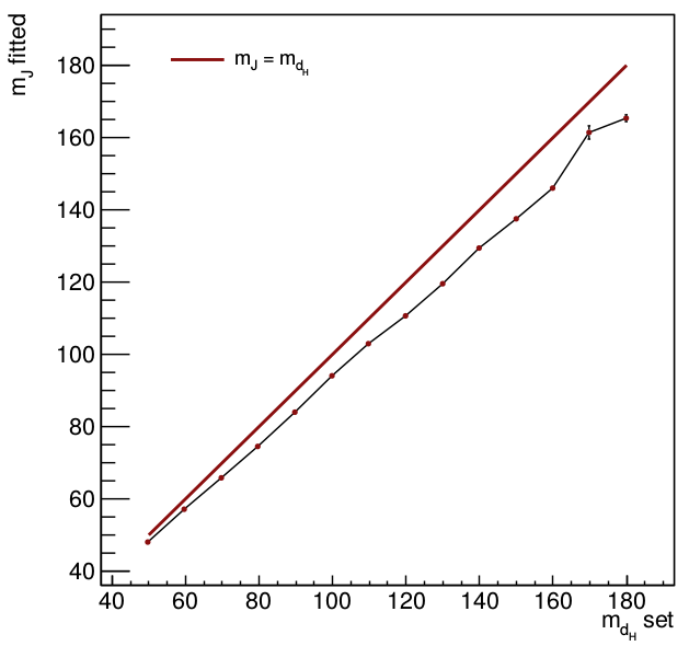
I've talked to Pedro and we concluded that the fat jet mass resolution is getting worse since the greater the m_{d_{H}} set, more non-collinear are the b's. To check that, I've tightened the MET cut (from 500 to 700), and we saw that the resolution got a bit better. A study about the efficiency of the cut may help with this problem. Also, this seems to be a characteristic of the jets and fat jets invariant mass resolution (the difference of m_{J} and m_{d_{H}} scales with the mass).
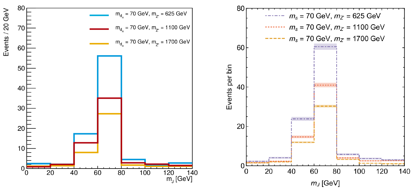
The macro
V9_terceiromais_dark_Higgs.C was also used at the processes with different m_{Z'} and the results were just as I've expected.
23/07/2019
All the macros are working perfectly. The macro
punzi_eff_lepcut.C needed to have the number of events exchanged, since the restriction in the lepton p_T made the cut looser (and the relative efficiencies were getting higher than 1). I must talk to Thiago about this.
I'm using the fat jet pt macro in all the other dark Higgs masses to see what happens to the efficiency. Luckily, it will change something. I'll also use the macro of the fat jet mass to analyze the events.
29/07/2019
I'm running all the macros again with the Z' mass variations, only to check what is happening. I still need to plot signal and background MET one over another to check if the MET efficiency is alright. If there is something missing, I can generate events with a looser cut in MET and merge it with the ones I already have.
30/07/2019
After running the macro to calculate the efficiencies of the MET cut, no important result was found, in the sense that the significance only goes down. I'll check why that is happening. Also, me and Thiago saw that some of the processes generated by the
MadGraph have a Higgs or a dark Higgs mediating the production of two b's and two DM particles. I'll see the lagrangian implemented inside the UFO files.
I've created a macro to plot the MET and the fat jet p_T in the same histogram to see what is happening with the Punzi significance. Thiago said that is important to have the BG separated being compared with the signal, but also the BG all together being compared with the signal. I've only rescaled the histogram by each of the processes cross sections. Later, I can normalize everything to see what happens. Thiago have showed me a variable that might be interesting to plot and cut it in some interesting region: \sqrt{2 * p_{T}^{J} * MET * (1-cos(\Delta \phi (J,MET)))}.
At tuesdays and wednesdays I'll start participating in the dark Higgs technical chat (tuesdays) and the monojet meeting (wednesdays). This will be very nice to learn a lot of new stuff with people that work in the same stuff that I'm doing right now.
I've generated histograms of the transverse mass, and it really seems that it can be cut to increase the significance of the search!!!
01/08/2019
Yesterday I've listened to the monojet meeting, and they were talking about some discrepancies in some monojet samples cross sections, that could be caused by the use of a wrong PDF.
Today, I've created a macro to analyze the Punzi significance of cuts in the transverse mass, and it really seems that awesome results will come out. I'll show this in today's SPRACE physics meeting. I think I should run the macros to the other masses as well.
The results from the Punzi significance for cuts in the transverse mass show a very small improvement in the significance for one of the cuts, and I'll show it in todays meeting. It's not a great gain, but it's something.
05/08/2019
At the 01/08 meeting, Pedro sugested that I should cut the M_{T} variable in a window around the Z' mass. Maybe I'll heva some gain in efficiency here. I don't remember exactly when, but I have written a macro to plot the cross sections of the processes for different m_{d_{H}} or m_{Z'}. It' named
plot_dh_xsec_wo_cuts.C (since it only has the
MadGraph +Pythia+Delphes generation cuts), and the files created were
xsec_mdh_var_nocuts.pdf and
xsec_mdh_var_nocuts.pdf.
I'll begin to create folders for each different macro that I'll use. All the files related to a test of that macro will be in subfolders inside the "master" one related to that macro. I hope that all my files get more organized in this way. The folder name will be exactly like the macro name.
06/08/2019
Yesterday I've showed to Thiago the results of the Punzi significance for the transverse mass cuts for the file with m_{d_{H}} = 70
GeV and m_{Z'} = 1100
GeV, and it wasn't very satisfying. Thiago asked me to do the same with a bigger m_{Z'} file, and I did for the 2000
GeV one, which got us even more confused. I'm using the LHE files to calculate the p_{T} of the sum of the four-momentum of the DM particles, and it's exactly like the MET in the root file corresponding to this mass.
The macro name is
read_fourvector.C, and there is a folder with the same name, with all the files/canvases of this macro.
09/08/2019
I've presented a summary of the CWR paper yesterday at the meeting, and already sent my comments/doubts to Pedro.
Thiago helped me to realise that there was an error in the macro
read_fourvector.C. I've fixed it, and inside the folder
read_fourvector, there is another folder with the name
macro_certa, where all the right plots are, including a figure that compare the MET histograms for different values of m_{Z'}.
Today me and Thiago had a talk about what should I do in the next few weeks, and these are my tasks:
*Build a table with all the number of events;
*Build a cut flow for some (all) of the m_{D_{H}} values;
*Learn how to use ROOT TLimit or TRolke (or both);
12/08/2019
I've modified the macro
punzi_eff_bg_separated to find the best window around the best center value (that I got through the highest Punzi significance). The files are inside the folder
best_punzi_center_varying_binsize in the folder named after the macro. Now, I'll modify it to find the number of events of signal and BG after all the cuts, in the region of highest Punzi significance for the center and the window, and it will be named
punzi_eff_table_cutflow.C.
There were some errors in the tables, and I'll se what is happening tomorrow. But it seems that I'm at the right way.
14/08/2019
The first table is below. The number of events is normalized to a luminosity of 140 fb^{-1}
| m_{d_{H}} [GeV] |
N_{S} |
N_{B} |
m_{J}^{center} [GeV] |
m_{J}^{window} [GeV] |
| 50 |
77.8346 |
59.5086 |
50 |
20 |
| 60 |
101.74 |
47.6723 |
58 |
16 |
| 70 |
136.038 |
68.2943 |
66 |
20 |
| 80 |
166.037 |
122.624 |
74 |
28 |
| 90 |
172.762 |
136.005 |
82 |
28 |
| 100 |
175.813 |
140.486 |
98 |
36 |
| 110 |
174.741 |
131.641 |
110 |
40 |
| 120 |
166.938 |
105.836 |
112 |
36 |
| 130 |
122.976 |
87.6493 |
122 |
32 |
| 140 |
104.722 |
136.891 |
130 |
44 |
| 150 |
57.0858 |
165.731 |
146 |
44 |
| 160 |
18.6357 |
271.383 |
150 |
72 |
| 170 |
3.43249 |
250.224 |
160 |
64 |
| 180 |
2.07056 |
218.363 |
166 |
56 |
Some examples of cutflow are
I can't understand why the Punzi significance or the number of events statistical significance is getting lower after each cut.
19/08/2019
Today I've been working on the suggestions everyone gave me at last thursday's SPRACE physics meeting. I'm still not sure about the Punzi significance getting lower, and I'll Thiago to show him these results. I've also changed the calculation of BG for the Punzi significance to the expression that Ana and Tulio are using that is the sum of the efficiency times the cross section times the luminosity of each BG separately, but it didn't changed much in the results. I'll talk to someone about this and check what is the right expression.
I've created a new macro called
punzi_eff_table_cutflow_lepbef to check what happens if I do the lepton veto before the MET cut, and how this changes the Punzi significance.
I've created a macro to test the TLimit class from ROOT. It's named
tlimit.C and it uses the ROOT file
140_fb_newbin_xsecfactor_ATLAS_kfactors_NLO_bgchange_mais_certo_ALL_bg_sig_70gev_withiso.root since it already have 140 fb^{-1} of luminosity and it has BG + Sig to test. I'm still very confused about this class, and what its outputs represents for the dark Higgs model. But I've only tested with one mass, and I must do it to the other masses as well.
I'm doing the poster for ENFPC, and I'll get some stuff from the previous poster. I might put something about the validation of the model (following the dark higgs paper) and some of these efficiencies/significances results.
20/08/2019
In the folder
NLO_mais_certo_ALL_backgrounds_combined_rightratio are the histograms that compare the fat jet mass of BG only, signal only and BG+sig for all the m_{d_{H}} values. I'll use those to test TLimit and TRolke. The files are named
140_fb_newbin_xsecfactor_ATLAS_kfactors_NLO_bgchange_mais_certo_ALL_bg_sig_"+m_{d_{H}}+"gev_withiso.root.
I've created a macro to test the TRolke ROOT class, that is named
trolke_example.C, that is in its ROOT class reference. I'm still trying to figure out what to do with this, and what efficiencies should I use in my case. Also, what is the ratio between signal and BG regions.
27/08/2019
Today I've talked to Thiago, and I'm testing the TLimit ROOT class only using some number of events. For now I've done for 3 events, 5 events and 10 events, in 8 different cases: (sig, bg, data) = (0,0,0); (n,0,0); (0,n,0); (0,0,n); (n,n,0); (n,0,n); (0,n,n); (n,n,n). Actually, I need to use 0.0000000001 events to represent 0, since I was getting some error messages.
I'll start doubling the last case data number of events, to see what happens (I'm expecting that CLs and CLsb will increase as n is higher).
29/08/2019
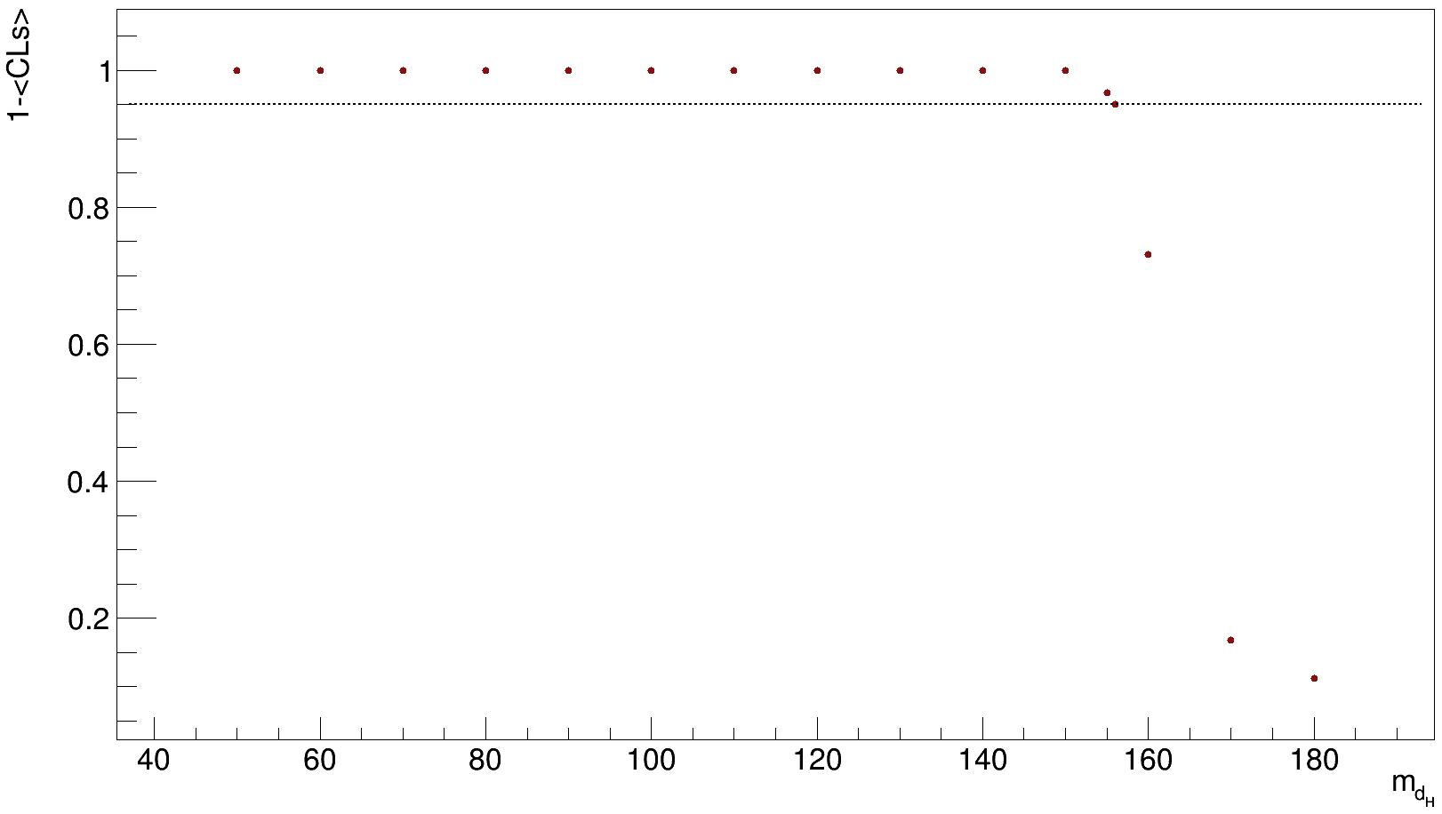
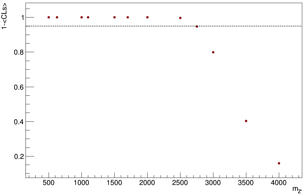
I've tested the TLimit class, and it works reasonably good. Using it, I could set exclusion masses for d_{H} and Z'. The table for the number of events for each m_{Z'} is (the luminosity was set to 140 fb^{-1})
| m_{Z'} [GeV] |
N_{S} |
N_{B} |
m_{J}^{center} [GeV] |
m_{J}^{window} [GeV] |
| 500 |
228.074 |
68.2943 |
66 |
20 |
| 625 |
216.908 |
68.2943 |
66 |
20 |
| 1000 |
142.014 |
68.2943 |
66 |
20 |
| 1100 |
136.038 |
68.2943 |
66 |
20 |
| 1500 |
128.621 |
68.2943 |
66 |
20 |
| 1700 |
101.867 |
68.2943 |
66 |
20 |
| 2000 |
67.6939 |
68.2943 |
66 |
20 |
| 2500 |
28.3811 |
68.2943 |
66 |
20 |
| 3000 |
11.3235 |
68.2943 |
66 |
20 |
| 3500 |
4.58453 |
68.2943 |
66 |
20 |
| 4000 |
1.72912 |
68.2943 |
66 |
20 |
The graphs are below. Everything above the dashed lines is excluded with more than 95% CL.
- cls_mdh.png:
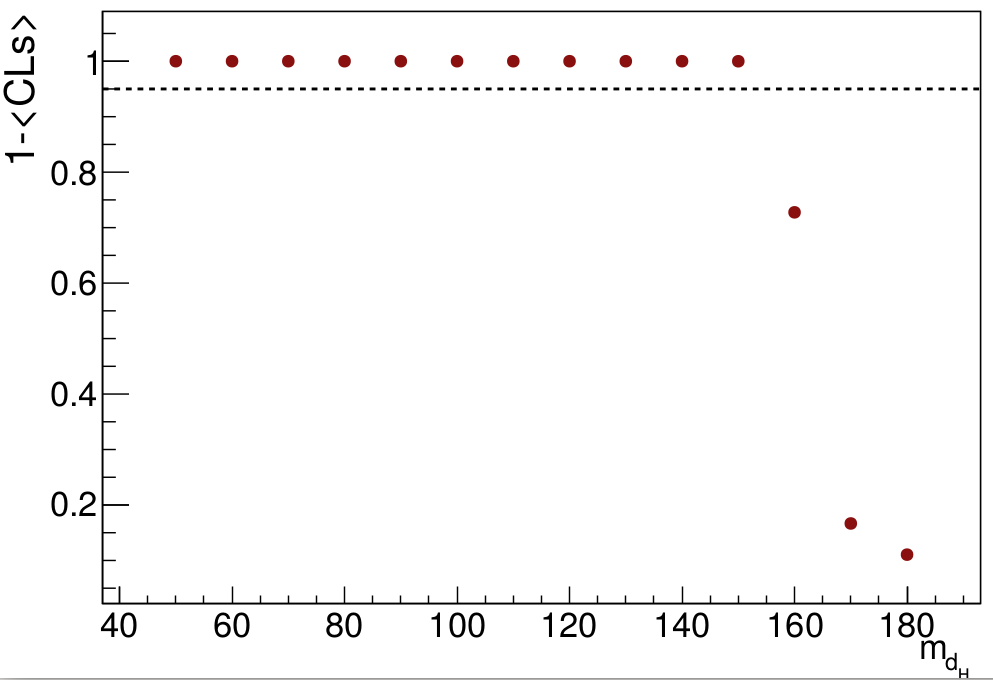
- cls_mzp.png:
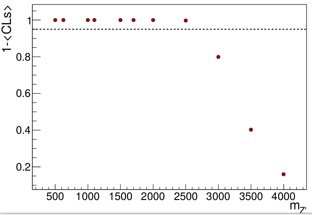
In the first plot it was set m_{Z'} = 1100
GeV and m_{\chi} = 100
GeV. In the second plot it is m_{d_{H}} = 70
GeV and m_{\chi} = 100
GeV.
06/09/2019
This was ENFPC 2019 week. While there, I learned how to make my DM particle look like a neutrino for the
MadGraph misset generation cut. Now I can run only 5k events with a MET restriction, instead of 300k events without MET restriction, and obtain the same result. The change was in the
SubProcess/setcuts.f file, where the line
if (abs(idup(i,1,iproc)).eq.1000022) is_a_nu(i)=.true. needs to be added after the same lines but with the neutrinos PDG codes. This will improve my results a lot.
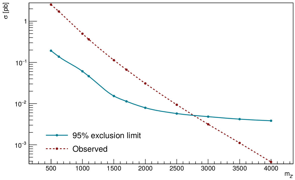
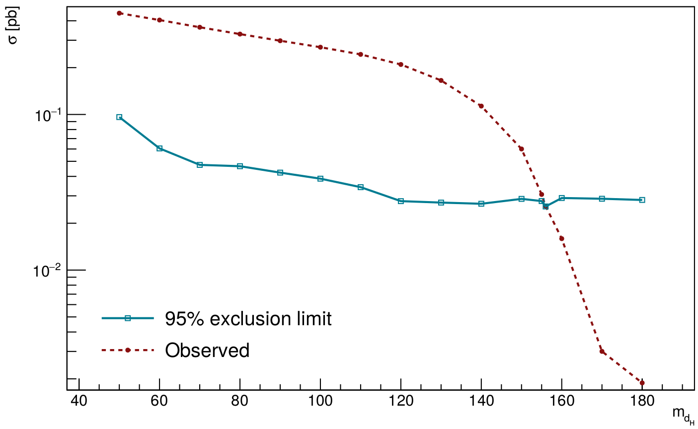
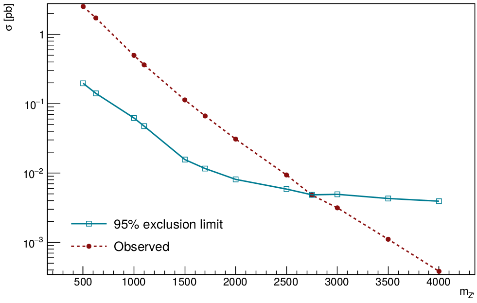
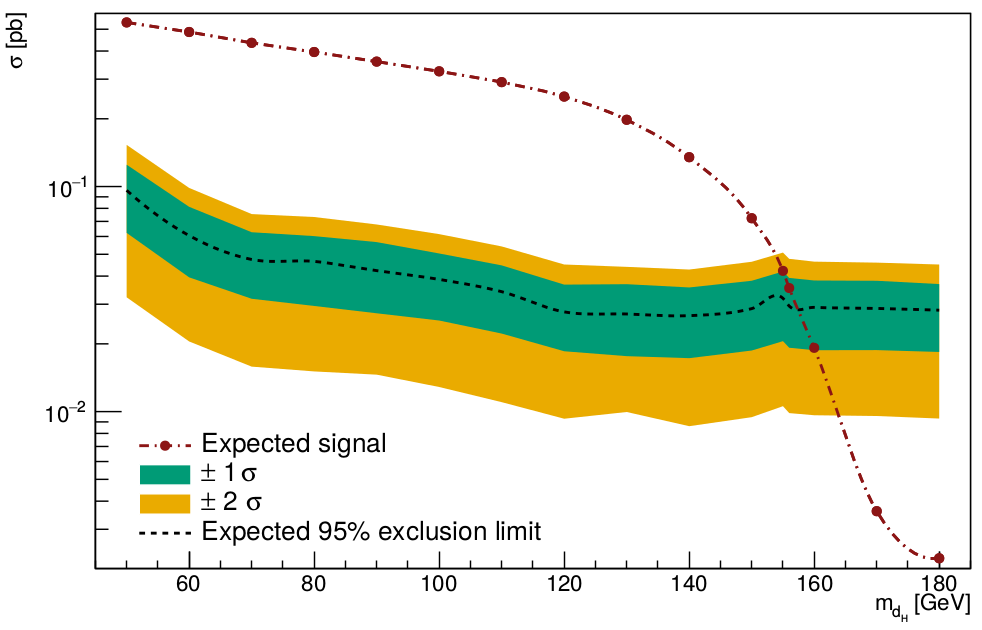
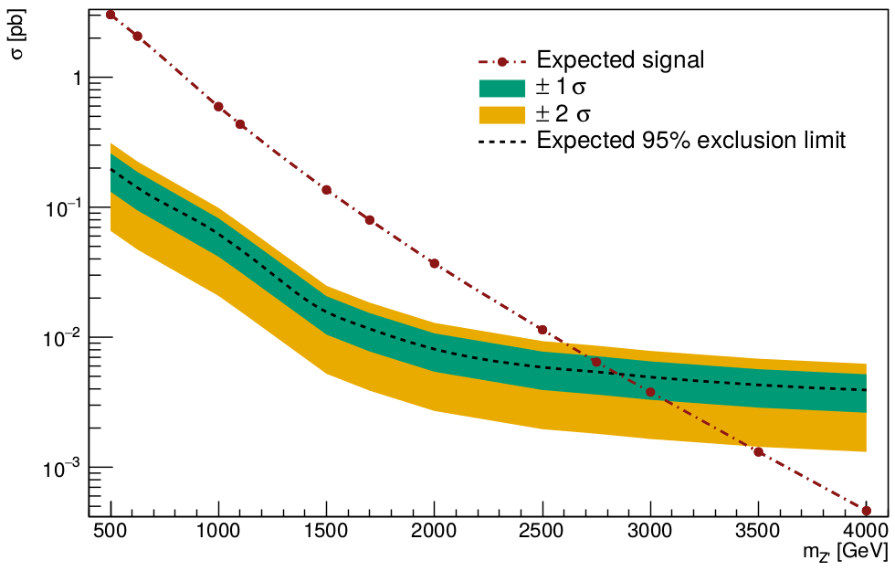
Today I did what Thiago told me to a couple of weeks ago. For each value of m_{d_{H}} and m_{Z'}, I needed to find the number of events N that gave me almost 95% CLs (actually 1-\<CLs\>) using the TLimit ROOT class, and calculate the cross section for that value using the formula
\sigma = N/(lumin x eff). Then I would calculate the cross section using the number of events that I've found for each m_{d_{H}} or m_{Z'} concerning each BG, and compare both. The graphs are below. Everything that is above the blue line, is excluded with 95% certainty.
- mdh_xsec_cl.png:
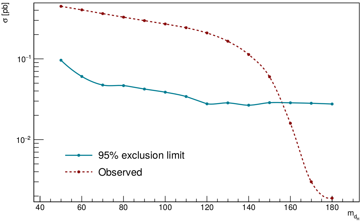
- mzp_xsec_cl.png:
10/09/2019
Today I'll start generating new mass points for the CLs plot, to get the exact point in which the curves will cross each other, for different m_{d_{H}} and m_{Z'}. Also, I'll check the difference in the CMS cards with and without pile-up from Delphes.
I'll run the events locally, since they can be running while I do other stuff. Only a couple of thousands of events (10k is enough I guess) will be generated for each point, since I've learned how to make the misset cut in the generation of the signal processes.
In the folder
Template/LO/SubProcesses/ inside the MG5 folder, I've found the file
setcuts.f. Maybe, changing that file will change all the other ones that will be newly created. I've tested it, and it actually works! This will make everything easier, even when running thing in access2, since ther I can't change anything inside a folder before running a given process.
I've generated the mass point
m_{d_{H}} = 155 GeV, and, since all d_{H} files in the Delphes folder are named as
mais_certo_300k_*gev.root, I'll name the root file as
mais_certo_300k_155gev.root (even though it has only 10k events). The cross section of this process was
0.00567 pb (because of the MET cut).
The step-by-step from going to the root file, to a point in the CLs graph is as follows:
- Use the macro V10_terceiromais_dark_Higgs.C to check the m_{J} variable;
- Find the best value of the Punzi significance for the m_{J}^{C} and m_{J}^{W} using the macro punzi_eff_bg_separated.C;
- Get the number of events of signal and BG in that region, and the efficiency using the macro punzi_eff_table_cutflow.C;
- Use the macro tlimit_mdh_mzp.C with those number of events to find 1-CLs;
- Find the 95% number of events for that given N_{BG};
- Convert everything to xsec using the expression \sigma = N/(lumin x eff), and multiplying the efficiency by 1.2 * xsec (with MET cut)/xsec (without MET cut), with the macro tlimit_to_xsec_mdh_mzp.C.
The informations for the mass point 155
GeV are:
To rescale the cross section, I've calculated it by simulating in
MadGraph the same process without the MET cut (since all the other points in the graph has this restriction), and the result was
0.06797 pb. An important point, is the 1.2 factor from madgraph in the final result. To find it consistently with the other points, this factor needed to be taken into account.
The 155
GeV mass point didn't touch the 95% exclusion limit, and I'll try to simulate the 156
GeV one (it was already very close).
I've found the 1.2 factor inside the
MadGraph folder, and it's just a
grep "1.2" *.f inside Template/LO/Source to see it. This factor doesn't appear in the NLO processes.
11/09/2019
I've already simulated the 156
GeV m_{d_{H}} without MET cut to calculate the cross section, and the result was
0.05776 pb. Today I'll also do the same thing with the Z' masses.
The process with the MET cut have a cross section equal to
0.004846 pb. The file in the Delphes folder is called
mais_certo_300k_156gev.root.
The informations for the mass point 155
GeV are:
The plot with the new points is below
- xsec_mdh_155_156.png:
I've simulated the mass point m_{Z'} = 2750
GeV, that have a cross section equal to
0.01159 pb (without MET cut) and
0.002832 pb (with MET cut). The file in Delphes folder is named
mais_certo_300k_2750gev.root. The results for this mass point are
The plot with the new point is below
- xsec_mzp_2750.png:
The new 1-CLs plots are below
- cls_mdh_com_intermediarios.png:
- cls_mzp_com_intermediarios.png:
17/09/2019
Today I've studied the difference between the Delphes CMS cards with and without PU. Apparently, the particles (including the ones coming from PU) have no correction until the end of the calorimeters. After that, the first correction (PU track correction) is applied, which will interfere in the jets (that have another correction: jet PU correction) and in the isolation of electrons, muons and photons. This means, that almost all of the Delphes outputs will have corrections in the end. An interesting feature is that there isn't a module for the
FatJets. I guess I'll introduce it by hand and check what is the difference (in practice) to the card without PU. There is a flowchart that shows the steps that Delphes makes while working. It's inside my main folder, and it is named
delphes_PU_finished.png.
I've also looked inside the Pythia files to write very clearly what are the processes that it's seeing while simulating the signal processes. In
MadGraph syntax, the following 6 different processes were found:
- q ~q > H* > hs n1 n1, hs > b ~b;
- q g > H* q, H* > hs n1 n1, hs > b ~b;
- q ~q > Z'* > hs n1 n1, hs > b ~b;
- q g > Z'* q, Z'* > hs n1 n1, hs > b ~b;
- q ~q > hs* hs, hs* > n1 n1, hs > b ~b;
- q g > hs* hs q, hs* > n1 n1, hs > b ~b;
Particles tmarked with * are the ones that have its mass very close to the m_{Z'} set in
MadGraph param_card. It's interesting that only those particles are decaying to the 2 DM, even when we have 2 intermediate dark Higgses.
Today I've started looking the TLimit class to see how to put uncertainties in the BG. Apparently, it's just use the syntax
TConfidenceLevel * TLimit::ComputeLimit (Double_t s, Double_t b, Int_t d,
TVectorD * se,
TVectorD * be,
TObjArray * l, Int_t nmc = 50000, bool stat = false, TRandom * generator = 0), where s, b and d are signal, BG and data, respectively, se and be look like the errors per bin of the signal and BG histograms (in my case that will be only a number), I don't know what is l, nmc is the number of montecarlo simulations to do, stat is dependent on the shape of the number of events (if I want to count one tail of the distribution, or none of them) and the generator is the random generator. I've also discovered how to find the results of TLimit with +/- 1 and +/- 2 sigmas (the default is 0, the average). I'll try everything out.
I'm having some problems to implement the BG errors in TLimit. The classes
TVectorD and
TObjArray are a bit weird, and I'll talk to Thiago tomorrow to see how to do it. In the mean time, I'm thinking if it's suitable to only vary the number of events in the BG for some different values like 10%, 20%, and some others, and see how the CLs variable will change, and how this affects the cross sections.
I can do the same thing with the -2, -1, 0, 1 and 2 sigma expected CLs, converting everything to number of events of signal and than to cross sections (would this be a brazilian plot?).
18/09/2019
Today me and Pedro checked the class about statistics. Everything seems clear, and the exercises were extremely helpful to understand different types of CL calculations, especially when it talked about the CLs method (since I had no clue of what it was doing). I'll prepare something for the next week meeting.
I'm also working on a macro to write the results of TLimit with 1 and 2 sigmas. It's named as
tlimit_testes.C. The other important macro of today is the
tlimit_tlimit.C, where I'm testing the uncertainties in the signal and BG values. Unfortunately, the TLimit calculation with histograms without uncertainties is not equal to the TLimit calculation with double values. I've checked that, and what was happening was that I forgot to turn off the statistical uncertainties when I was comparing both of them. I'll ask Thiago if it's important to account for both uncertainties right now.
I've created the macro
brazilian_not_brazilian_plot.C with the 1/2 sigmas values, and already updated the macro
tlimit_to_xsec_mdh_mzp.C to plot that graph. It is very impressive, but I don't know how to make it beautiful for now. I'll show this plot and some results at tomorrow's meeting.
20/09/2019
Yesterday, while talking to Pedro, we saw a little divergence in my macros. I was using MG5 luminosity to perform all the calculations until the tlimit macros. Unfortunately, the correct luminosity is achieved by using the expression
L = N/xsec. But madgraph gives me 2 numbers for each of those quantities. The first one is the number of events in the run_card (that I set to do the Monte Carlo simulations), and the xsec assigned to the process concerning thi number of events and a fixed luminosity. The other ones are the number of events after pythia matching/merging and the xsec assigned to that number of events, that provide the same luminosity as the numbers before. Since Delphes is using the later, I needed to change the luminosity that I was calculating using
Lnew = N(after matching/merging) / xsec (after matching/merging). This shall not change the results significantly, but it will make the cross sections calculated through TLimit and the MG5 ones more consistent.
I've already compared the m_{J} graphs from the paper with the ones using this new quantity to validate this case, and it seems pretty good.
The new xsecs (after matching/merging) for the different values of m_{d_{H}} are:
| m_{d_{H}} [GeV] |
approx x-sec [pb] |
| 50 |
0.536 |
| 60 |
0.486 |
| 70 |
0.435 |
| 80 |
0.396 |
| 90 |
0.359 |
| 100 |
0.325 |
| 110 |
0.291 |
| 120 |
0.251 |
| 130 |
0.198 |
| 140 |
0.135 |
| 150 |
0.0723 |
| 155 |
0.00368 (w/ MET cut) |
| 156 |
0.00311 (w/ MET cut) |
| 160 |
0.0192 |
| 170 |
0.00361 |
| 180 |
0.00223 |
I still need to do the processes for 155 and 156 without the MET cut, but with pythia and Delphes to get the merged xsec.
The new xsecs (after matching/merging) for the different values of m_{Z'} are:
| m_{d_{H}} [GeV] |
approx x-sec [pb] |
| 500 |
3.030 |
| 625 |
2.069 |
| 1000 |
0.594 |
| 1100 |
0.435 |
| 1500 |
0.136 |
| 1700 |
0.0797 |
| 2000 |
0.0369 |
| 2500 |
0.0114 |
| 2750 |
0.00169 |
| 3000 |
0.00378 |
| 3500 |
0.00131 |
| 4000 |
0.000462 |
I still need to do the process for 2750 without the MET cut, but with pythia and Delphes to get the merged xsec.
All the BG xsecs are all right, I just need to put the 1.2 factor inside their k-factors.
23/09/2019
The cross sections for the processes with m_{d_{H}} of 155 and 156 without MET cut are
0.0422 pb and
0.0354 pb. For the m_{Z'} 2750 process it is
0.00643 pb.
04/10/2019
I'll stay at CERN for almost 3 months. While in here, I am going to work with Maurizio Pierini with Deep Learning applied to High Energy Physics. I'm reading the Deep Learning book (which is available at the web) and it seems pretty good for now. I must learn what is a Generative Adversarial Network (GAN) that is the last chapter of the book. Also, I am searching for some Machine Learning frameworks (mainly Keras with Tensorflow as backend, but I might change it to Torch since is what Raghav (Maurizio student I guess) is using) and how to work with MNIST datasets (the handwritten numbers and the fashion one). Everything is amazing, and I believe that this will be a major step for me.
While here, at fridays I will work on the dark Higgs model. Today I built the brazilian plot graphs again (but now some less ugly ones) that are:
- brazilian_mdh.png:
- brazilian_mzp.png:
I was not inserting the right errors in the
TGraphAssymErrors and that was a problem. But I've learned it now. I'll use TLimit with systematical errors in the BG now and see what happens. I am going to write a new macro for this, since the one that I was using is gone (something in my backup went wrong I guess). The new macro is named
tlimit_tutorial.C.
Thiago have made some test about it and he sent me the file with some results. The file is named as
ComparacaoTLimitCombine.xlsx and it is inside my Delphes folder. I'll also save it in the "home" of my flash drive and my external HD.
There are 24 images (12 for m_{d_{H}} and 12 for m_{Z'}) for the variation of systematic uncertainty. I don't understand some of the results, but I must show this to everyone and ask for some explanation. They are in the folder
tlimit_tutorial.
To gather better results, I've simulated more mass points for m_{d_{H}}, and I'll do the same for m_{Z'} also. For now the mass points simulated and their respective cross sections are:
With metcut
Without metcut
The files inside Delphes folder are named as
mais_certo_300k_* just for simplicity. For m_{Z'} the xsecs are:
With metcut
| m_{Z'} [GeV] |
approx x-sec [pb] |
| 2050 |
0.005976 |
| 2100 |
0.005443 |
| 2150 |
0.004983 |
| 2200 |
0.004664 |
| 2250 |
0.004201 |
| 2300 |
0.003878 |
| 2350 |
0.003529 |
| 2400 |
0.003191 |
| 2450 |
0.002887 |
| 2550 |
0.002404 |
| 2600 |
0.002255 |
| 2650 |
0.002037 |
| 2700 |
0.001857 |
| 2750 |
0.001679 |
| 2800 |
0.001537 |
| 2850 |
0.001406 |
| 2900 |
0.001278 |
| 2950 |
0.001150 |
Without metcut
| m_{Z'} [GeV] |
approx x-sec [pb] |
| 2050 |
0.03253 |
| 2100 |
0.02939 |
| 2150 |
0.02551 |
| 2200 |
0.0232 |
| 2250 |
0.02019 |
| 2300 |
0.01808 |
| 2350 |
0.01579 |
| 2400 |
0.01433 |
| 2450 |
0.01295 |
| 2550 |
0.01025 |
| 2600 |
0.009138 |
| 2650 |
0.008178 |
| 2700 |
0.007278 |
| 2750 |
0.006527 |
| 2800 |
0.005934 |
| 2850 |
0.005372 |
| 2900 |
0.004714 |
| 2950 |
0.004222 |
19/02/2020
While at CERN I've got some nice results by using a
ConVAE to generate jets. There is a lot of work ahead (learn what are and how to use the energy flow polynomials), but I think we are in the right track.
Concerning the Dark Higgs model, a lot of advances were made. First of all, the brazilian plots of m_{d_{H}} and m_{Z'} are very nice and I learned how to use TLimit with systematic uncertainties in the BG (useful in the future, or to be more familiar with other methods). Thiago gave me access to headtop, and this is helping a lot on the simulation of new data. With it I was able to reproduce (badly) the left image of figure 5 from the "Hunting the dark higgs" (arXiv:1701.08780) paper, below
In headtop, the files
steering* and
param_card_* inside MG folder are the mass points being used for m_{d_{H}} = 70
GeV. I am doing m_{\chi} = 50 -> 800
GeV (50) and m_{Z'} = 250 -> 4000
GeV (250), 120, 3200, 3400, 3600 (more resolution is needed). The exclusion region applying only the MET > 500.0
GeV cut for L = 150 fb^-1 is almost identical to the paper one for L = 40 fb^-1. With m_{J} cuts, the exclusion region is highly improved, but I don t know if this cut could be used in a real analysis. Also, inside each of the folders for the mass points, called
teste_MET400_*, inside the
Events folder, where all the root files are,
the merged_xsec.C will get the cross sections after merging, that is the right one.
In headtop, inside the Delphes folder, the important macros are
ultimate_* for each of the cuts, and every result is inside the folder
testezao separated in each cathegory. I am getting the exclusion region for L = 150 fb^-1 (run 2), L = 300 fb^-1 (end of run 3, predicted), L = 1000 fb^-1 (end of run 4, predicted), L = 3000 fb^-1 (end of LHC, predicted).
In my computer there is also a folder named
testezao, and the results are in the
top folder. Three macros inside the Delphes folder are important
plot_top_xsecs.C,
plot_top_xsecs_lumi.C,
only_plot_top_xsecs_lumi.C. They make these graphs
I am finishing the BEPE report. I am waiting for a feedback from Thiago about the latest version, and then I will need to ask for a letter from Maurizio.
14/04/2020
I've been working on my master dissertation. I am finishing Thiago's corrections. Everything is almost done, there are just a few things to work on. I need to generate the cross section graphs from the files
xsecs_* inside Delphes folder in my computer (they are also at my area in headtop, inside the folders named
plot_xsecs). The macro to generate those graphs is
plot_xsecs_mzp_mdh_mdm.C.
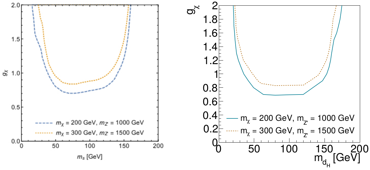
There are other macros to plot the exclusion reginos inside delphes folder that are
plot_top_xsecs_lumi_interpolation.C,
only_plot_top_xsecs_lumi.C and
only_plot_top_xsecs_every_lumi.C. The files that I need are at/ are being created at the
testezao/top/ folder. In headtop, every
ultimate_* macro inside the Delphes folder is analyzing the events generated by
MadGraph. They are named as
400MET_*. There are events for fixed m_{d_{H}} with m_{Z'} and m_{\chi} varying, and for fixed m_{Z'} and m_{\chi}, for m_{d_{H}} and g_{\chi} varying. The results are in agreement with the paper.
- mzp_mchi_excl_comp.png:

- mdh_gchi_excl_comp.png:
01/10/2020
I've been working with the FIMP model. Its simulation using
MadGraph + Pythia + Delphes (going to call it just Delphes for simplicity) is not that good, since there are a lot of electrons/muons missing. Eduardo suggested that this is happening because of a generation cut (
MadGraph or Pythia or even Delphes) that I am going to investigate. I am also trying to simulate it using the
FullSim of CMSSW, but it might be harder.
The Delphes generated events are in the folder
~/MG5_aMC_v2_6_6/FIMP_leptons_varying_width. An important macro is in the Delphes folder under the name
Delphes_FIMP_hist.C and some results are in the folder
Delphes_FIMP. 10000 events were generated for each decay width value with m_{F} = 130
GeV, m_{s0} = 125
GeV and from run_01 to run_10 the decay length (c\tau) is approximately 100 mm, 200 mm, ..., 1000 mm and runs 11, 12, ..., 15 are 2 m, 4 m, 8 m, 16 m, 32 m respectively. Run_16 is a prompt (setting the decay width to 1) test. In
MadGraph the syntax to simulate the events is p p > he~ HE~, and the F decay is being performed by Pythia through changes in the SLHA table. The tracks transversal impact parameter seems to be what I expected, however, the number of reconstructed (generated) electrons + muons that is around 1100 (7600) is much lower than the ~ 20000 expected from the Fs decay. I need to test a few things to find out where the problem is:
- Change the s0, F mass difference to see if events that contain leptons with higher p_T are sufficient (this would point to a generator cut that might be caused by Madgraph, Pythia or Delphes)
- Check the number of s0 generated particles (if this number is 20000, this would point only to Pythia or Delphes, I guess)
- Check the reco and gen leptons p_T (this is not that useful since I would expect only leptons that already passed MadGraph lepton p_T restriction)
- Check gen particle status (from Pythia log they must be +/- 23)
The number of generated s0 with status 23 is equal to the number of generated electron + muon with status 23.
The status of every s0 is equal to 23 (and there are status=0 that I don't know what it means).
MadGraph has a selection cut on leptons p_T of 10
GeV. This shouldn't be a problem since
MadGraph would then generate events that have laptons p_T around this value.
Delphes imposes an efficiency of 0 in reco leptons that have p_T < 10
GeV (great issue concerning the mass difference that I set).
Gen leptons have very low/high p_T, and reco ones have p_T > 10
GeV from the cut I described before.
In run_17 I set m_F = 300
GeV and m_{s0} = 125
GeV with c\tau ~ 200 mm to see if the problem with the leptons would continue (I didn't change any generation restriction in Madgraph or Pythia or Delphes). The number of generated s0 and electrons + muons are equal ~ 11000, but they are much lower than the expected (~ 20000). However, the number of reconstructed electrons + muons is around 15000 which is a great improvement. This was due to the Delphes restriction on leptons p_T indeed.
Run_18 is the same as the above, but with only 100 events. I am going to check the hepmc file to see if there is any valuable information about why some s0 and generated electrons/muons are missing. The hepmc file showed that even though every s0 or lepton that comes out of the F decay appear there as a stable particle (status=1), not all of them have the hardest subprcess outgoing status (23). I am going to talk to Thiago about this (mainly about if I should fix it in the hepmc file (which would take a very long time) or how to get the right tracks).
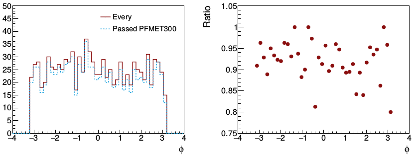
05/10/2020
With respect to my HLT studies, Thiago asked me to apply the PFMET300 trigger in some
NanoAOD file (I used a dark Higgs one) and to plot two histograms: one with every event MET and every event that passed the trigger MET; and the ratio of both (passed/every). These three plots and the \phi of the MET of the passed and every event MET (and their ratio) plots are in the images below.
- met_hlt.png:
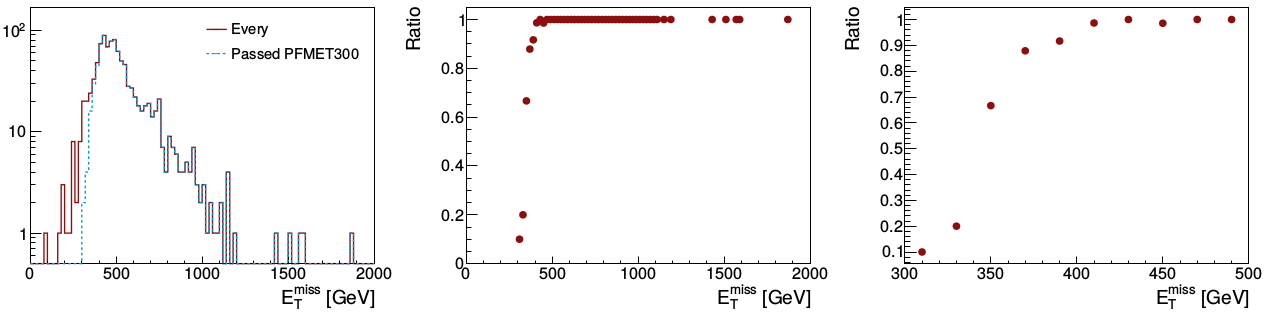
- phi_hlt.png:
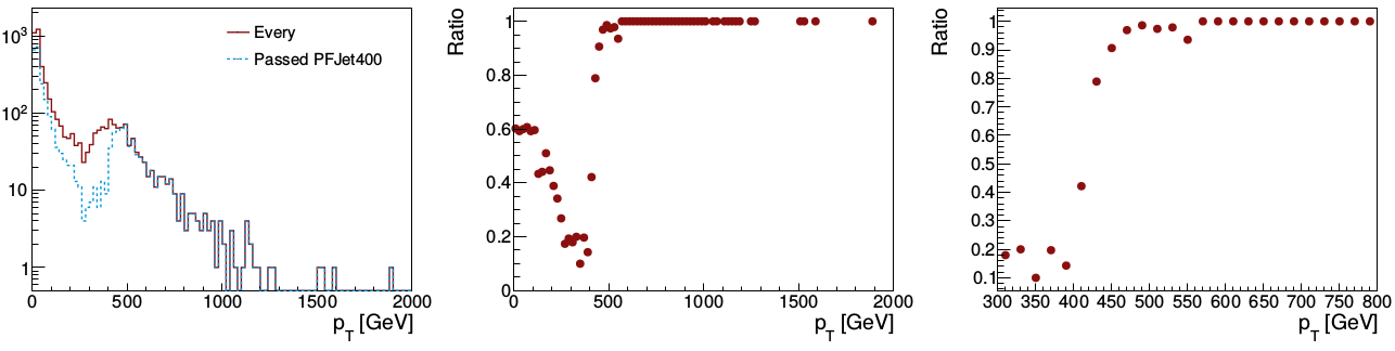
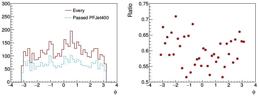
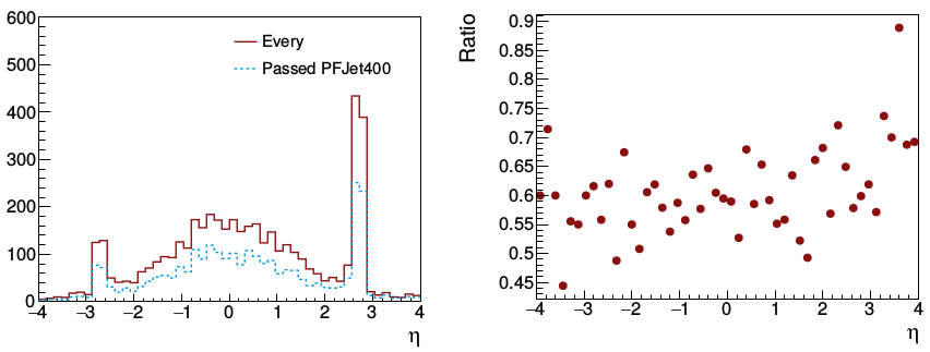
Today I did almost the same, but choosing a jet trigger (I am using the PFJet400 trigger in a drak Higgs
NanoAOD file; the dark Higgs events jets are recoiling against a very high MET, so they are boosted and have a very high p_T), and I need to talk to Thiago what he meant with matching offline and HLT jets (the information I have fromt he trigger is just which event passed the trigger or not; I don't have any information about the reconstructed objects during the HLT step).
- jet_pt_hlt.png:
- jet_phi_hlt.png:
- jet_eta_hlt.png:
07/10/2020
I am back at working with FIMP model using Delphes. The histograms of the D_0 of the tracks of electrons/muons (Delphes tracks have a member function called PID since it have access to the generated particle; this might be a matching between generated particle and track (need to investigate it just to make it more clear)) follow the expected. However, I used the files with 10000 generated events with the low F, s mass difference, which doesn't provide a lot of reconstructed electrons/muons. I am going to generate more of those events, but setting m_F = 300
GeV and m_{s0} = 125
GeV, and also changing the decay width. I am also going to set Delphes to reconstruct the F tracks, which is going to be useful for a few of the model's signatures.
In the folder
FIMP_leptons_varying_width_bigmdiff_wFtrack, run_01 is for promptly decaying F, run_02 - run_11 are F with c\tau of 100 mm, 200 mm, ..., 1000 mm, and runs 12, 13, ..., 16 are 2 m, 4 m, 8 m, 16 m, 32 m respectively. However, I forgot to put the output HSCP tracks in the Delphes card and all of them failed to give me a root file. I fixed it and I am trying to run again. It might not work though, since the input to the
ParticlePropagator module is all the stable particles that Delphes have access to, and F is not a stable particle (as I remember from the tests that I made on 01/10/2020; need to check it again). I built another Delphes module called
ParticlePropagatorHSCP where the input are all particles that Delphes have access to (all gen particles), and I am just picking the HSCP tracks to throw into the other modules (tracking efficiency and momentum resolution). I also had to add it in this file
ModulesLinkDef.h inside the modules folder. From run_17 to run_22 I have only failed tests (different configurations of the delphes_card.tcl and the modules). Run_23 was the one that worked, and I still need to test the properties of the F tracks.
I tested to run the decay in
MadGraph changing the time_of_flight variable of the run_card.dat and it actually worked. I don't need to put the F decay in the SLHA table for Pythia8, which is much easier. In folder
FIMP_test_runtofchange are two runs: run_01 that have c\tau ~ 1000 mm and run_02 is a promptly decaying F, and the difference of the D0 of muons (I only set them to decay into muon + s0) of both files is very big (prompt has basically all muons with D0 ~ 0).
In folder
FIMP_leptons_varying_width_bigmdiff_wFtrack_corrected, run_01 is for promptly decaying F, run_02 - run_11 are F with c\tau of 100 mm, 200 mm, ..., 1000 mm, and runs 12, 13, ..., 16 are 2 m, 4 m, 8 m, 16 m, 32 m respectively with F being a track. I am going to use these files to test the tracks.
13/10/2020
I checked the status of the leptons and s0 after generating the decay of F in
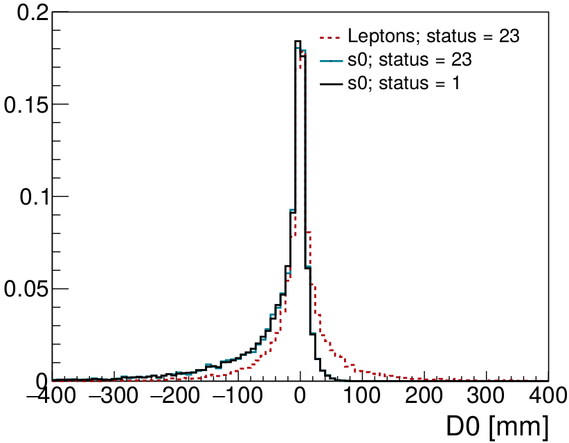
MadGraph (through p p > he~ HE~, (he~ > l- s0), (HE~ > l+ s0)), but I still have particles that have only status 1 and particles that go out with status 23 that is shifted to a status 1 particle. However I found out something more strange than that. Even though a lepton and a s0 share the same F parent, their D0 (I am getting this D0 as the generated particle D0; only the generated particles with PID = 255 or 11 or 13 with status = 23 that I am sure that come from the same F (this part I need to be sure if I am getting the right particles)) distribution is not the same. The s0 D0 distribution is not symmetric (the majority of the values fall in the D0 < 0 side) and the leptons D0 distribution is symmetric with respect to D0 = 0. I need to plot the quantities used to calculate D0 to see what is happening.
- D0_particles_em_s0.png:
16/10/2020
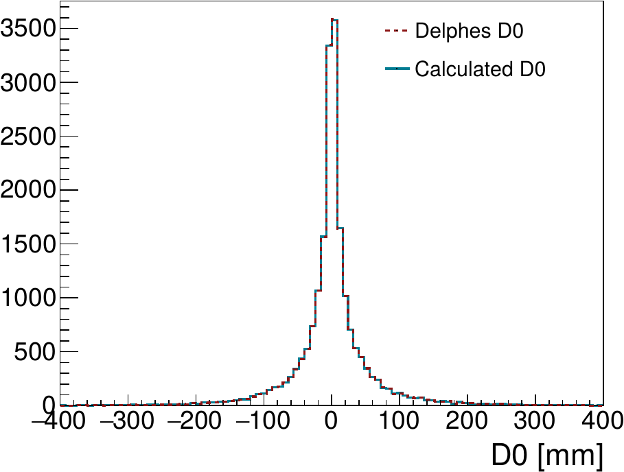
Apparently Delphes was calculating the D0 of the s0 particles wrong. Left plot below shows the comparison of all the leptons and s0 with status 1 that are daughters of F particles (there are 20000 of each), but with D0 being calculated as D0 = (x*py - y*px)/pt of the particles. Just to make sure that this equation is the one that Delphes uses, in the right plot I compared the distribution of the leptons D0 variables that comes from Delphes (lepton->D0) and the one calculated. They are exactly the same, with very few exceptions for very high D0 (I still need to make the same test with higher c\tau runs; this one is for c\tau ~ 100 mm).
- D0_particles_em_s0_Fparents_D0calc.png:
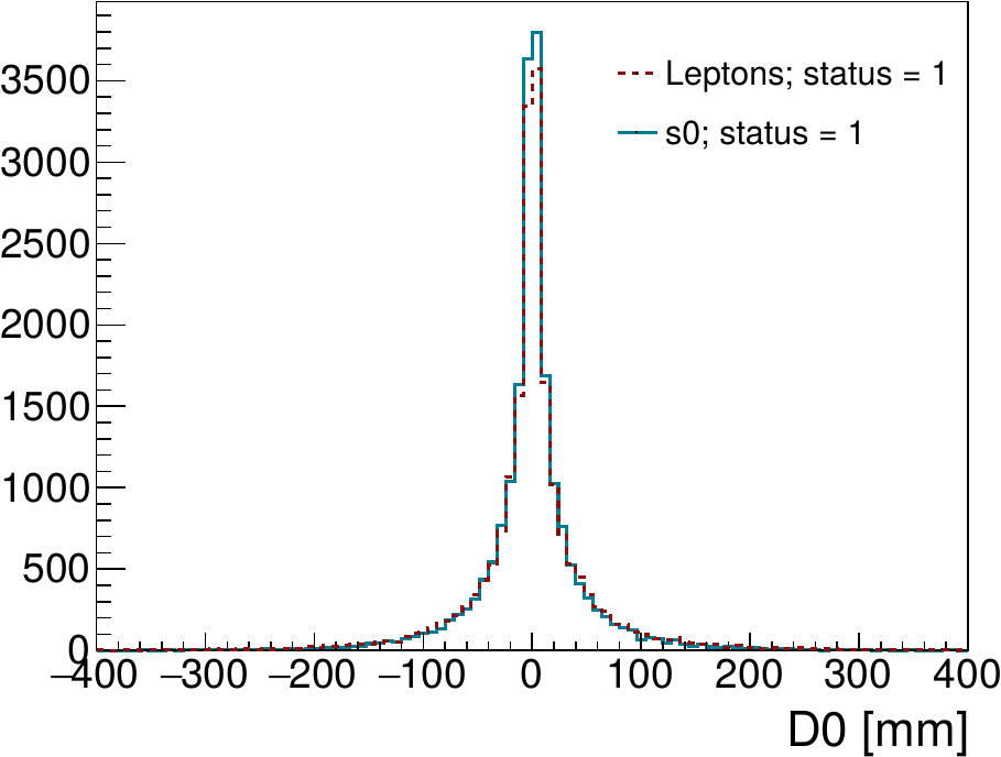
- D0_particles_em_s0_Fparents_lepcomp.png:
 , but it need to be changed to https://github.com/borzari/cmssw/compare/master...cms-sw:master


